


Hey guys, here’s this week’s edition of the Spatial Edge, a place where every join is a spatial join. Anyway, the aim as usual is to make you a better geospatial data scientist in less than five minutes a week.
In today’s newsletter:
Map Making: A field guide to turning ML models into maps.
Slum Mapping: Radar texture separates informal settlements from formal neighbourhoods.
Foundation Models: ESA pits TerraMind against THOR on ten tasks.
Generalist VLMs: A general model beats specialist designs with 80,000 samples.
SAR Reasoning: FUSAR-R1 reasons step by step over radar imagery.
Research you should know about
1. How to turn a machine learning model into a map
Image: Sialelli et al., arXiv
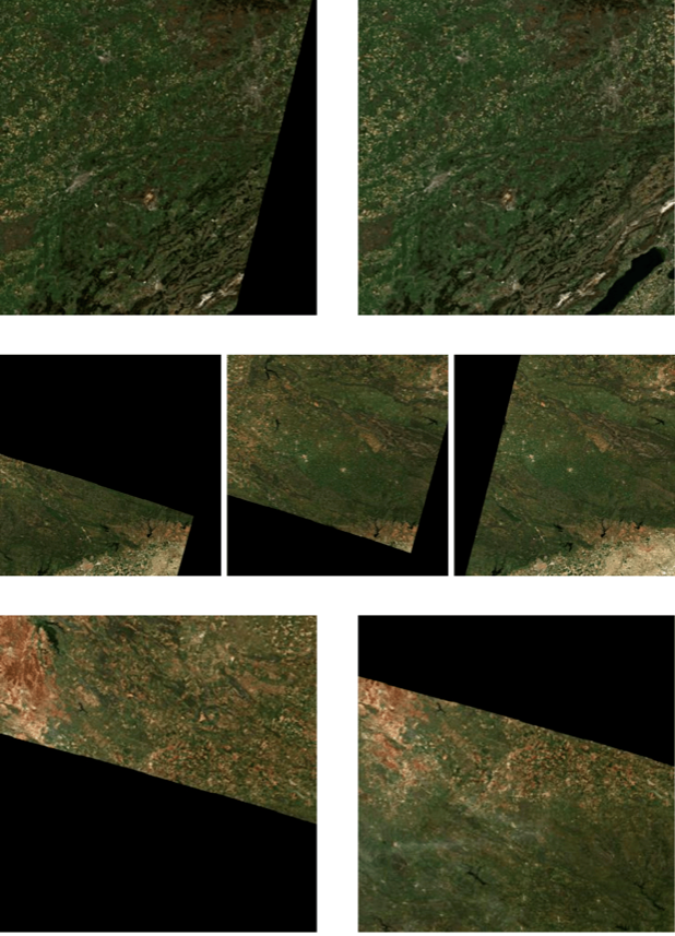
A new paper led by ETH Zurich, with co-authors from Cambridge, WSL, Asterisk Labs and a dozen other groups, sets out best practices for getting from a trained model to a large-scale Earth observation map, and it’s the guide a lot of us wished existed a few years ago. The barrier to producing a wall-to-wall map has dropped a long way, but there’s still no agreed playbook, and decisions made early in the pipeline quietly propagate errors into the final product. It was presented at the ECCV 2026 TerraBytes workshop.
The paper walks through six coupled stages: the data infrastructure landscape, data selection and preprocessing, dataset construction and training, uncertainty quantification, map production and distribution, and validation. The details are where it earns its keep. Google Earth Engine corrects the Sentinel-1 GRD radiometric offset while ESA redistributes the product as is, so switching providers shifts your input distribution. Sentinel-2’s January 2022 processing baseline change, incomplete orbits and Landsat 7’s scan-line gaps all show up as seams if you don’t handle them. Whatever preprocessing you use in training has to be reproduced over the whole mapped domain at inference, so every extra step compounds deployment cost. Spatial autocorrelation inflates apparent accuracy unless you split with blocked cross-validation and buffers wider than the autocorrelation range.
On uncertainty, the authors are blunt that no method is simultaneously cheap, scalable and well calibrated, and that deep ensembles trained on the same spatially autocorrelated data tend to agree where they are collectively wrong. Convolutional encoder-decoders remain the workhorse for wall-to-wall inference because of throughput, even as foundation models gain ground. And a held-out test set only tells you about generalisation within your sampling distribution, so a real map needs a probability-based validation sample where every location has a known, non-zero chance of being checked, with accuracy reported from both the user’s and the producer’s side. There’s an expanded online guide that goes with the paper.
2. Mapping informal settlements with radar texture
Image: Chepkilot, Memar & Gamba, arXiv (Fig. 1)
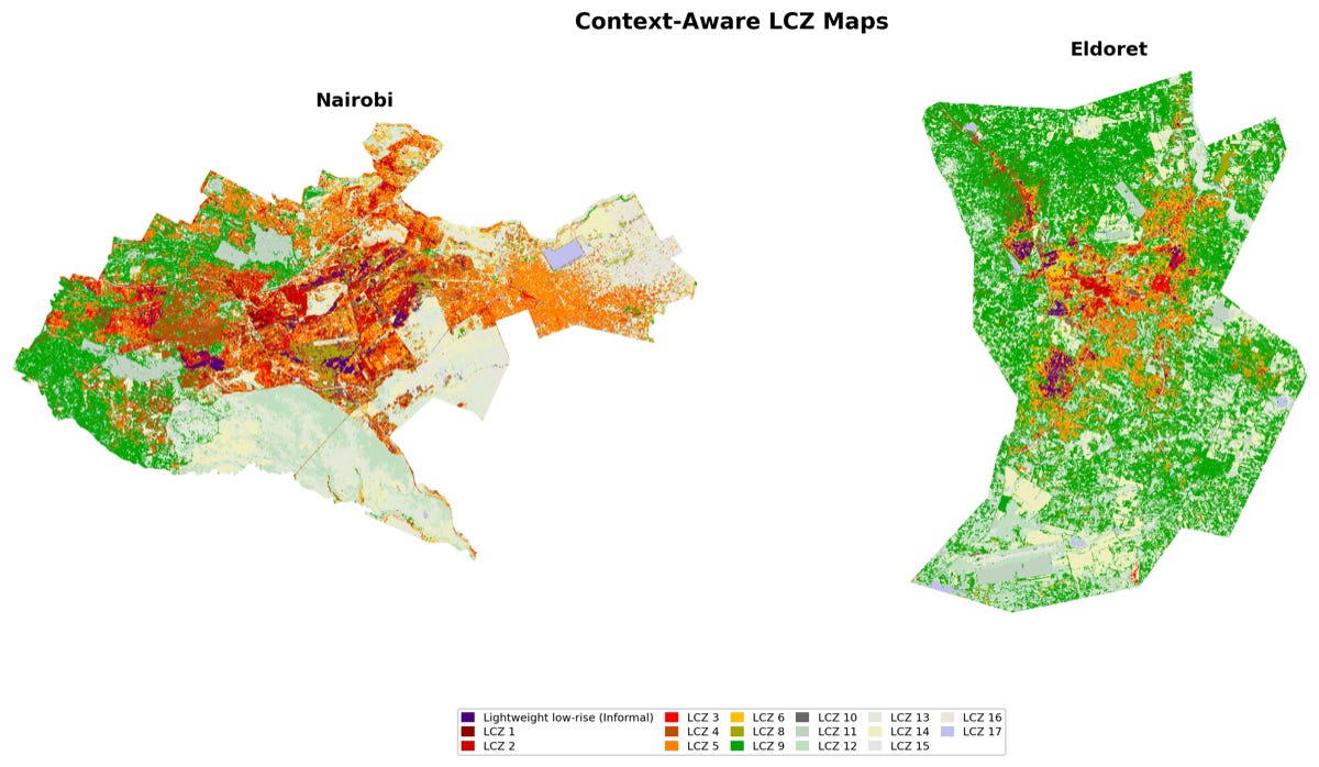
A new study from Sapienza University of Rome and the University of Pavia tackles a long-running problem in mapping Sub-Saharan African cities: from optical satellites, informal settlements look almost identical to formal, compact low-rise neighbourhoods. Both are roofed in the same oxidised corrugated metal, so reflectance-based classifiers confuse the two. The WUDAPT Local Climate Zone baseline mixes up the two classes 36.4% of the time.
The fix is to bring in Sentinel-1 radar in three tiers: calibrated VV and VH backscatter, grey-level co-occurrence textures over 3 by 3 pixel windows, and a physics-guided index that normalises VH entropy by mean backscatter power to pick out the high-disorder, low-return signature of lightweight low-rise housing. These sit alongside 18 Sentinel-2 indices in a 28-feature random forest, trained on 793 reference polygons in Nairobi and 492 in Eldoret (426,650 training pixels), with separate dry and wet season composites, and then tested on Kigali.
Adding the texture tier lifts overall accuracy from 70.4% for the WUDAPT baseline to 81.6% in the dry season, and the informal settlement F1 score more than triples, from 0.200 to 0.667. It also makes the map far less sensitive to season: the dry-wet F1 gap narrows from 0.084 with optical only to 0.004 with texture, and class confusion drops to 7.3%. The transfer test is the sobering part. Applied zero-shot to Kigali, overall accuracy falls to 0.363, and only with local labels added does the informal settlement F1 reach 0.720, so the features travel but the model still needs some labels from the target city.
3. ESA puts two Earth observation foundation models head to head
Image: Schindlegger et al., ESA Φ-lab, arXiv (Fig. 7)
A new study from ESA’s Φ-lab, IBM Research Zurich and the Norwegian Computing Center systematically compares TerraMind and THOR, the two geospatial foundation models ESA funded through separate consortia, across ten downstream tasks. TerraMind is a multimodal generative encoder-decoder pretrained on 500 billion tokens across nine modalities with a fixed patch size of 16. THOR is a vision transformer that accepts variable patch sizes from 4 to 32 at inference and unifies Sentinel-1, 2 and 3 at native resolutions.
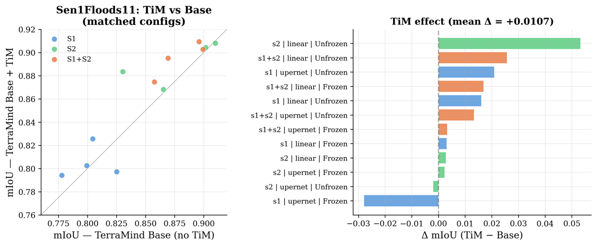
The benchmarks cover flood and burn scar segmentation, artisanal mining, methane leaks, soil property regression, iceberg detection, sea ice, snow and wetland mapping, with ablations over patch size, decoder type and frozen versus fine-tuned encoders, all run on a single RTX A6000. The headline pattern is that THOR leads on SAR-heavy and spatially compact targets while TerraMind leads on optical and multimodal ones, though the fine-grained results are more interesting than the leaderboard.
At matched compute TerraMind wins Sen1Floods11 with 0.910 mIoU against THOR’s 0.894, but THOR at patch size 4 hits an F1 of 0.86 on flood zone detection where TerraMind manages 0.33, and 0.873 mIoU on sea ice against 0.755, at 16 to 44 times the encoder cost. Patch size and decoder choice together explain more performance variance than which model you picked. Sentinel-2 alone beat Sentinel-1 plus 2 on Sen1Floods11 (0.910 versus 0.896), suggesting shallow fusion isn’t enough when optical signal is abundant, and THOR at 5% of the training data matched a UNet trained on 50%. The code is on GitHub.
4. A general-purpose VLM beats the remote sensing specialists
Image: Ailuro et al., INSAIT, arXiv
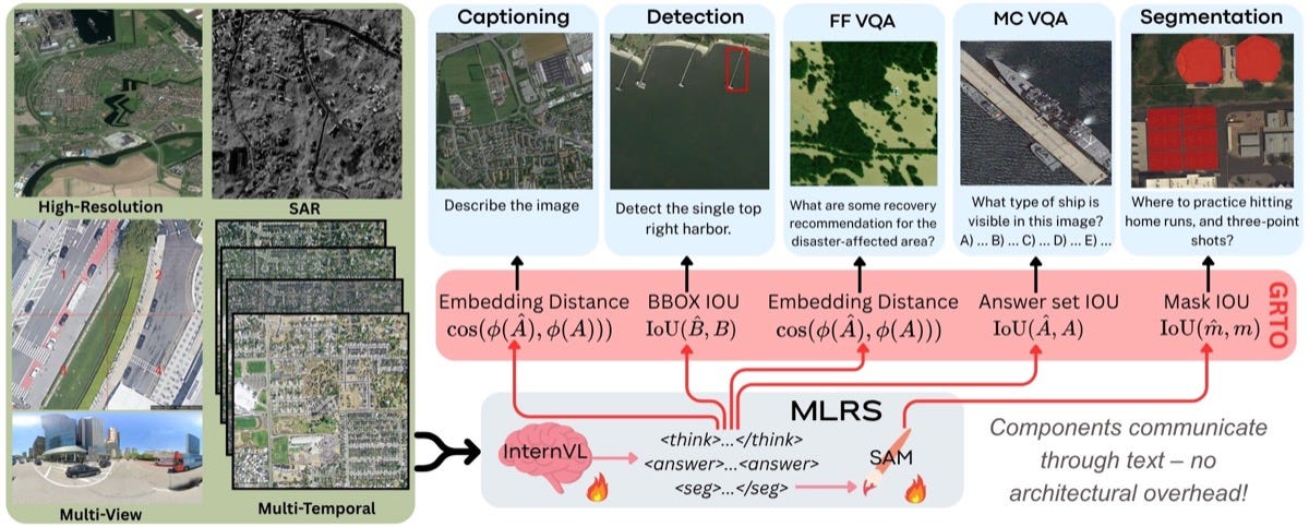
A new study from INSAIT at Sofia University, with Luc Van Gool among the authors, asks whether remote sensing vision-language models actually need custom encoders, alignment modules and task-specific fusion, or whether a capable general model with a good data recipe does the job. Most remote sensing VLMs lean on specialised architecture, which makes them hard to maintain and slow to benefit from progress in the general-purpose models.
The recipe is deliberately plain: take InternVL3.5 at 8B and 2B parameters, give it SAM3 as a segmentation tool, curate 80,000 training samples from a 2.3 million sample pool balanced across VQA, captioning, detection, segmentation, optical and SAR, multi-temporal, multi-view and very high resolution inputs, then fine-tune with LoRA for 5,000 steps using a group relative tool optimisation objective with task-dependent rewards. No remote-sensing-specific architecture anywhere.
On ten out-of-distribution benchmarks the model ranks first on seven and second on three, with detection precision at 0.5 IoU on GEOBench-VLM rising from 0.24 to 0.56, segmentation IoU on GeoSeg-Bench2 from 0.41 to 0.70, and a 7.6 times relative gain on XLRS-Bench detection. In-distribution it’s competitive or state of the art on DisasterM3, DynamicVL, SARLANG-1M and LaSeRS. The finding worth remembering is that performance tracked the diversity of data sources rather than sample volume: domains with three or more sources kept improving, while temporal VQA with two sources peaked early and then declined.
5. Teaching a model to reason step by step over radar imagery
Image: Yang et al., Fudan University, arXiv
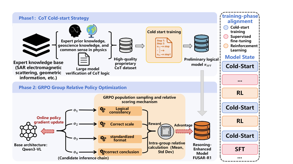
A new study from Fudan University introduces FUSAR-R1, a vision-language model for synthetic aperture radar that shows its working rather than jumping straight to an answer. Existing SAR VLMs output a label with no intermediate reasoning, no logical check and no way to self-correct, which matters when the physics of radar scattering is what separates a ship from a bright rock.
The team rebuilt the FUSAR-GEOVL-1M dataset so that each single-step description becomes a multi-step reasoning chain that folds in geographic context, scale priors, scattering feature analysis and spatial verification, with aircraft detection broken into seven steps and ship detection and land cover classification into six each. Training is a cold start of supervised fine-tuning on those chains followed by group relative policy optimisation with rewards for format, IoU-based detection, counting, classification and land cover recognition.
Against InternVL3.5-4B, FUSAR-R1 lifts object counting accuracy from 45.45% to 67.33%, main land cover category recognition from 44.23% to 85.24% and regional land cover from 6.55% to 64.75%, while cutting the land cover proportion error from 39.58 to 7.67. The ablation is the useful bit for anyone training these things: cold start plus reinforcement learning reaches a detection F1 of 0.676, cold start alone 0.600, and reinforcement learning on its own collapses to 0.197.
Geospatial Datasets
1. Every tree in New York City, by genus
Image: NYC Tree Genus Map (Miller et al., Cornell University)
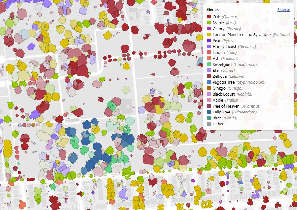
A Cornell team has classified 1.8 million individual tree crowns across New York City into 18 common genera, which together make up about 78% of the city’s basal area, using an XGBoost classifier trained on time series of 3 m PlanetScope imagery and airborne lidar structure, with labels extrapolated from the city’s street tree inventory. Overall accuracy is 82.0% (kappa 0.794), with Platanus at 95% producer’s and 93% user’s accuracy and Quercus at 88% and 80%, and around 1.4 million of the trees had never been surveyed before because they sit on private land or in natural areas. You can read the paper here, explore the interactive map here, access the data here and the code here.
2. Global evapotranspiration and GPP from 1982 to near present
Image: Earth System Science Data (Fig. 1)
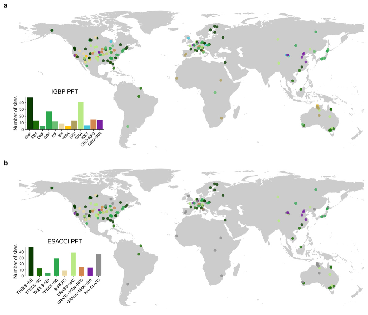
PML-V2.2 is a coupled evapotranspiration and gross primary production record in three flavours: 500 m 8-day from MODIS and VIIRS for 2000 to 2025, 0.1° half-monthly from AVHRR for 1982 to 2020, and a consolidated 0.1° series running from 1982 to 2025. The Penman-Monteith-Leuning model was calibrated at 208 flux sites (about 1,400 site-years) and separates irrigated from rainfed cropland, scoring NSE of 0.72 for ET and 0.76 for GPP at sites and 0.89 to 0.91 against basin water balances. You can read the paper here, access the data here or in Earth Engine, and the code here.
3. Daily temperatures from 17,000 stations on a common UTC day
Image: Earth System Science Data (Fig. 1)
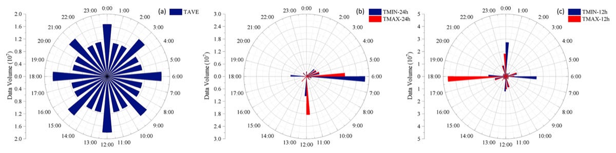
GLBD-FED provides daily maximum, mean and minimum temperature for roughly 17,000 weather stations worldwide from 1981 to 2024, all aligned to a 00:00 to 24:00 UTC window rather than each country’s local observing day. A reconstruction algorithm breaks the sub-daily Integrated Surface Database records into finer intervals and re-aggregates them, which recovers 64% more Tmax and 45% more Tmin values than the conventional approach, and daily coverage grows from about 3,000 stations in the 1980s to around 10,000 today. You can read the paper here and access the data here.
4. Corrected lightning events from China’s FY-4A satellite
Image: Earth System Science Data (Fig. 1)
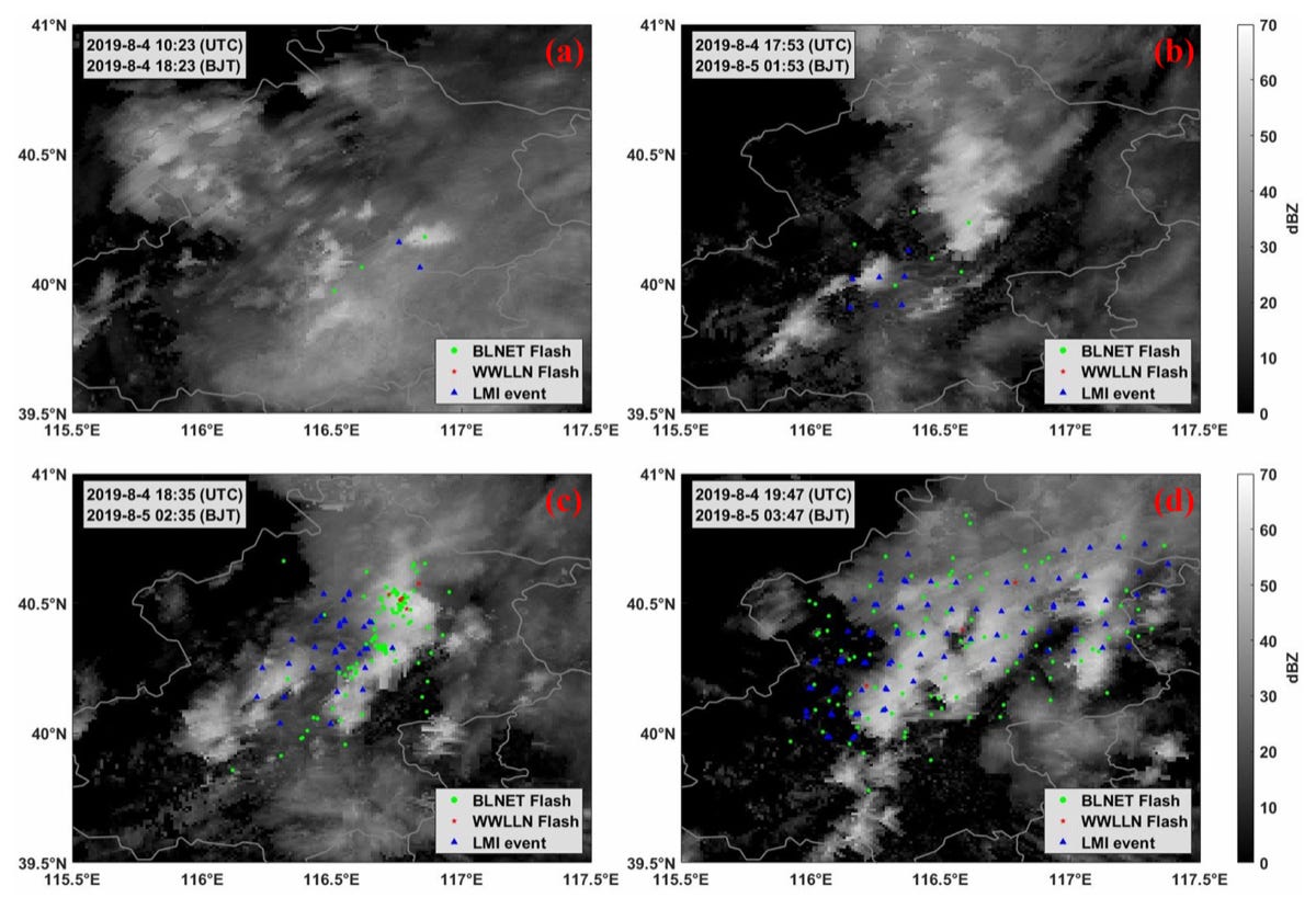
A geolocation-corrected event dataset from the Lightning Mapping Imager on FengYun-4A, covering the March to September warm seasons of 2019 to 2023 over China, Mongolia, Kazakhstan, Southeast Asia and surrounding seas at 7.8 km nadir resolution. Using the World Wide Lightning Location Network as reference, a spline correction applied across 400 subregions at 10-minute intervals raises the share of events within 15 km of their true position from 36.0% to 51.7%, and within 20 km from 58.2% to 74.8%. You can read the paper here and access the data here.
5. Seventeen years of solar-induced fluorescence from GOME-2
Image: Earth System Science Data (Fig. 1)
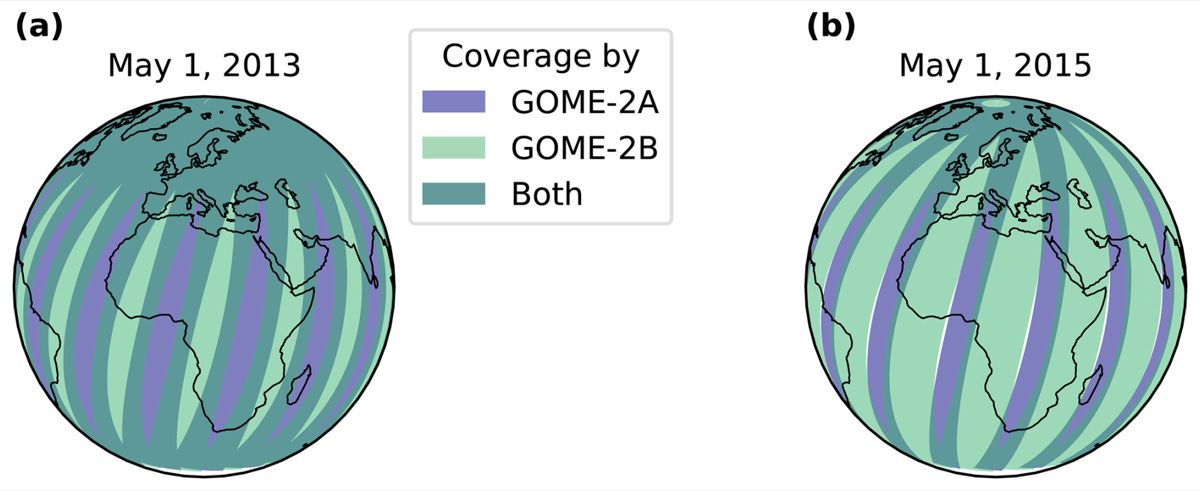
A combined solar-induced chlorophyll fluorescence record from the GOME-2A (2007 to 2017) and GOME-2B (2013 to 2023) instruments, gridded at 0.5° between 60°S and 60°N from native 40 km pixels, using the SIFTER v3 algorithm with time, wavelength and scan-angle dependent degradation corrections so the two sensors line up. You can read the paper here and access the data for GOME-2A here and GOME-2B here.
Other useful bits
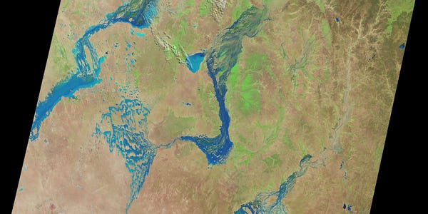
NASA has issued the request for proposals for the Landsat 10 spacecraft, with launch no later than 2031. The observatory will carry a single integrated sensor suite called LandIS, fly at 653 km with an 18-day global revisit, and catalogue scenes under a new WRS-3 reference system. Proposals closed on 13 August, the award is expected on 30 December 2026, and there’s a USD 1 million incentive for early delivery.
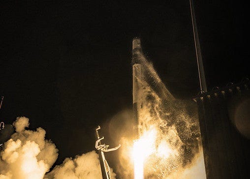
Rocket Lab has launched the ninth QPS-SAR satellite for Japan’s iQPS into a 575 km orbit from New Zealand, on Electron’s 93rd flight. iQPS is building out a synthetic aperture radar constellation aimed at 24 satellites by May 2028, and still has nine more dedicated Electron launches booked to fill it out by 2030.
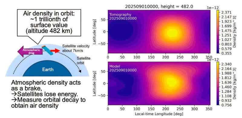
A Kyoto University researcher has used public Starlink orbital data to map the upper atmosphere, treating roughly 1,200 satellites at 482 km as drag sensors and applying tomography to infer thermospheric density, then checking the result against ESA’s Swarm mission. The paper in Earth, Planets and Space calls it a preliminary, low-resolution first map from a single week of data, but it’s a neat repurposing of a constellation nobody launched for science.
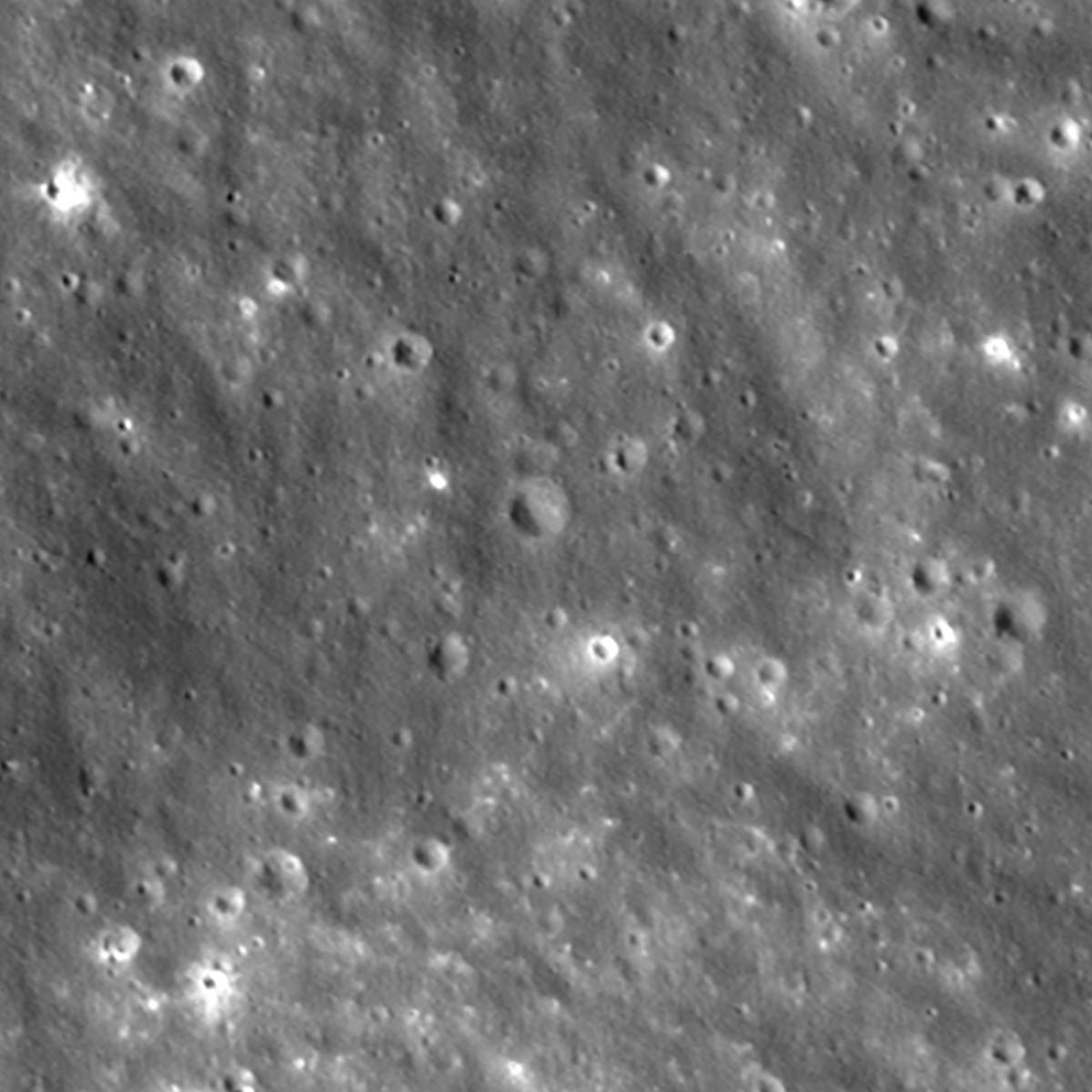
NASA’s Lunar Reconnaissance Orbiter has imaged the crater left by a Falcon 9 upper stage that hit the Moon on 5 August. Before-and-after shots from 11 and 12 August show a crater about 18 metres wide and under 3 metres deep, with dark rays of space-weathered surface material and brighter ejecta dug up from deeper down. Impact prediction tools, cross-checked with Korea’s Pathfinder Lunar Orbiter, got the location right to within about a kilometre.
Jobs
UNITAR is looking for an Individual Contractor – Geospatial Analysts – Satellite Imagery and GIS based remotely.
Esri is looking for an Imagery Product Engineer II for imagery and remote sensing based in Redlands, California.
Esri is looking for a GIS Product Engineer II for the ArcGIS Maps SDKs for Native Apps based in Cardiff, UK.
Mapbox is looking for a Machine Learning Engineer III working on routing cost based in Germany.
Overstory is looking for an Engineering Manager for Machine Learning, remote across the US, Canada and much of Europe.
Just for Fun
Image: Eddie Sgarbossa, via NASA APOD
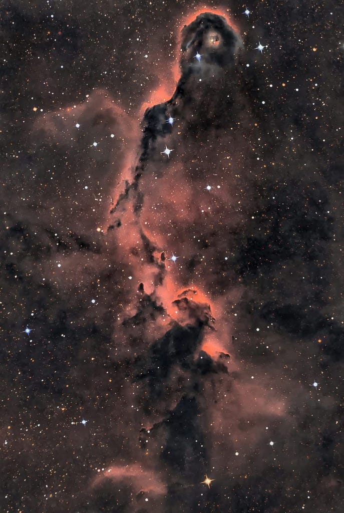
The Elephant’s Trunk Nebula winds through the emission region and young star cluster complex IC 1396 in the constellation Cepheus, about 3,000 light-years away. The trunk itself, catalogued as vdB 142, is more than 20 light-years long, and its bright ridges and dark, tendril-shaped clouds of cool dust and gas are the raw material for new stars, with protostars already hiding inside. The whole IC 1396 complex spans more than 5 degrees of sky; this view covers close to 1 degree, a little under the width of two full Moons.
That’s it for this week.
I’m always keen to hear from you, so please let me know if you have:
new geospatial datasets
newly published papers
geospatial job opportunities
and I’ll do my best to showcase them here.
Yohan