Tutorial: Downloading and processing Black Marble nightlights data in R

Part 2: A walk through on using Black Marble and Google Earth Engine with R

Yohan

Dec 27, 2023

Today’s newsletter provides an in-depth tutorial on processing nightlights images using R.

If this isn’t up your alley, you might like some of my less-technical posts on X over the last week such as:

Onto the tutorial:

Today, I’ll be showing you:

how to process Black Marble nightlights imagery in R; and
how to process Colorado School of Mines’s nightlights imagery from Google Earth Engine (also using R).

This is Part 2 of my series on nightlights data. If you haven’t already, check out Part 1, which provides the background to all of the steps we’ll be taking.

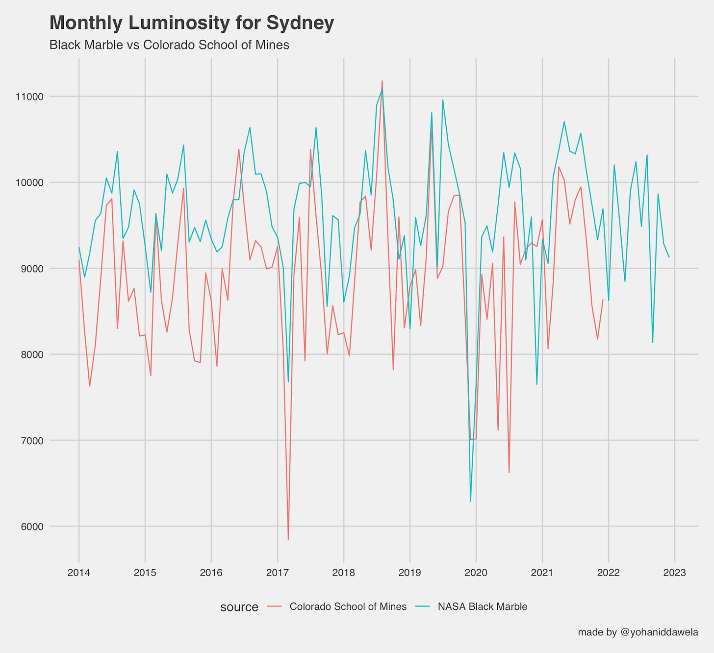
By the end of this tutorial, you’ll be in a position to create a graph like this, which plots Black Marble and Colorado School of Mines monthly nightlights data:

This post contains screenshots of the codebase, but the full codebase will be emailed exclusively to subscribers of this newsletter on Friday 29 December 2023.

This will be a once off only, so make sure you’re subscribed if you want to receive it.

Section 1: How to process Black Marble data

As we saw in Part 1, Black Marble nightlights data isn’t as easy to process as Colorado School of Mines’s off-the-shelf product.

It used to be an absolute nightmare to process Black Marble images for a region of interest. I was previously using packages like httr, sf, raster, gdalutils, rgdal, and set up a bunch of custom functions.

However, Rob Marty and Gabriel Vicente have released two amazing packages, which make the process significantly easier:

For the sake of this article, I’ll be focussing on the blackmarbler package for R.

Alright, now let’s begin with setting up the Black Marble workflow.

Step 1: Sign up for NASA’s Earth Data platform

Go to https://urs.earthdata.nasa.gov/home and then fill out your details and click register.

Step 2: Go to NASA’s LAADS DAAC site

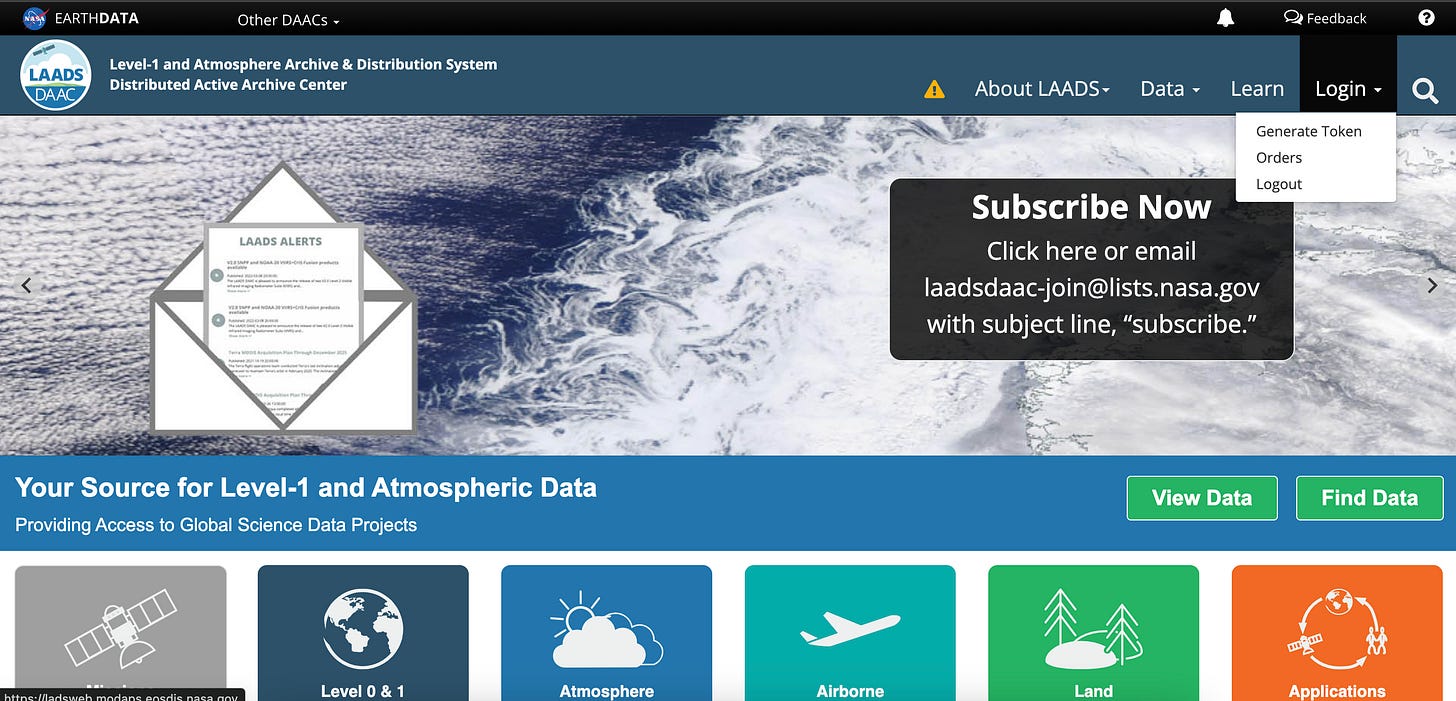
Now go to: https://ladsweb.modaps.eosdis.nasa.gov/ and click the ‘login’ drop down on the top right.

Now click ‘Generate Token’, and copy the token text.

This text is called your ‘bearer’. We’ll be using it to connect to Black Marble’s database via API in the next step.

Step 3: Set up your R script

Before getting started, make sure you have the following packages installed:

sf, terra, blackmarbler, raster, exactextractr, lubridate, geodata

Then save your bearer token in the script (I usually save these as environment variables, but for the sake of this tutorial, we’ll be saving them directly in the script).

Step 4: Get your region of interest

In this example, I want use Sydney, Australia as the region of interest.

So I call the following function from the geodata package to obtain the shapefile for Sydney.

Step 5: Download the Black Marble data

In this step we’ll be:

downloading monthly Black Marble data (this has the product ID: VNP46A3)
dropping cloud-contaminated pixels and bad-quality observations
selecting the date range we’re interested in
selecting whether we want off-nadir, near-nadir or all-angles (see Part 1 for more information on these)
adjusting for snowfall

In this example, I’ll be using monthly luminosity data from January 2014 to December 2022, all-angles, and ensuring that snowfall has been controlled for.

Step 6: Imputing missing values

Because we’ve dropped cloud contaminated pixels, we have a bunch of pixels that have no values. We therefore need to impute their value.

We can do this by looking at the value of previous months and future months, and then linearly interpolate the missing pixels.

This can be programmed as follows:

And there you are. You now have a raster stack full of Black Marble luminosity data that’s controlling for factors like snowfall, cloud cover, seasonal vegetation, etc.

The next step is to conduct zonal statistics so that we can create a line graph.

Step 7: Zonal statistics

Here, we calculate zonal statistics to sum up all luminous pixels within Sydney and create a data frame:

The end result is a data frame that looks something like this where:

GID_2 is the unique ID for Sydney from the shapefile; and
Luminosity is the sum of all luminous pixels within Sydney

Step 8: Create line graph

Now we can create a line graph of luminosity using the ggplot2 package.

Simply use the following code:

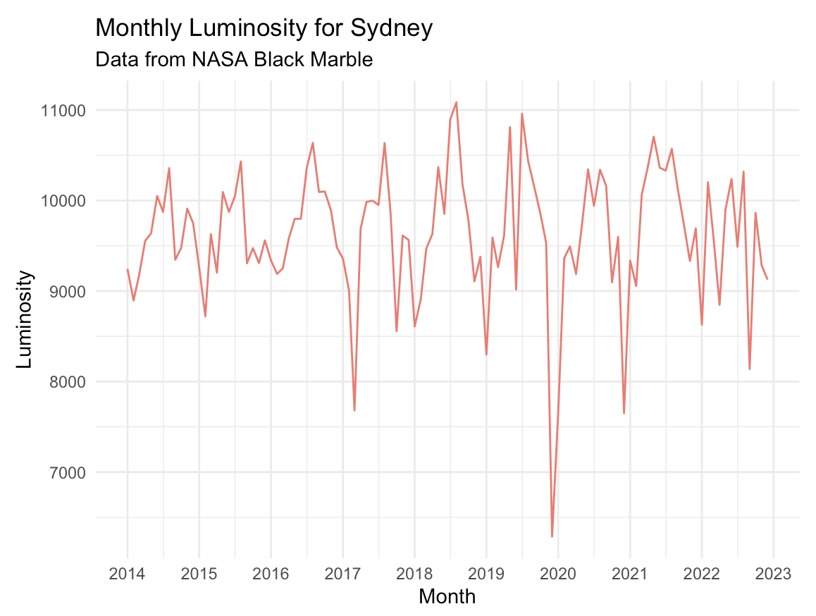
And the output will be the following:

Section 2: How to process Colorado School of Mines data from Google Earth Engine

Step 1: Install the RGEE package on R

Getting the RGEE package can be a bit fiddly, so I recommend watching the following video to get set up:

Step 2: Load packages and initialise Google Earth Engine

You’ll need to have the following packages installed.

rgee, sf, tidyverse, geodata, raster, reticulate, lubridate

Now load them as follows, and initialise GEE:

Step 3: Get your region of interest

We follow the same instructions from Step 4 in Section 1.

This provides us with an SF object for Sydney.

Step 4: Import the nightlights dataset

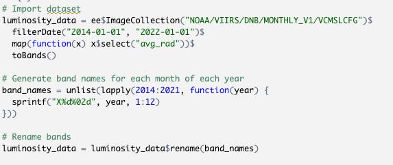
For this, we’ll be using monthly nightlights data from Colorado School of Mines. This has the GEE Image Collection ID of: "NOAA/VIIRS/DNB/MONTHLY_V1/VCMSLCFG".

Make sure you’re using the stray light corrected dataset from GEE.

We can import the dataset in R as follows. This loads monthly luminosity data from January 2014 to December 2022.

Step 5: Calculate zonal statistics on GEE

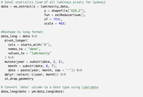
We’ll be using the ee_extract function to sum up all luminous pixels in Sydney.

We’ll then be creating a long data frame, which tracks monthly luminosity for Sydney (from January 2014 to December 2022) as per the previous step.

The code is as follows:

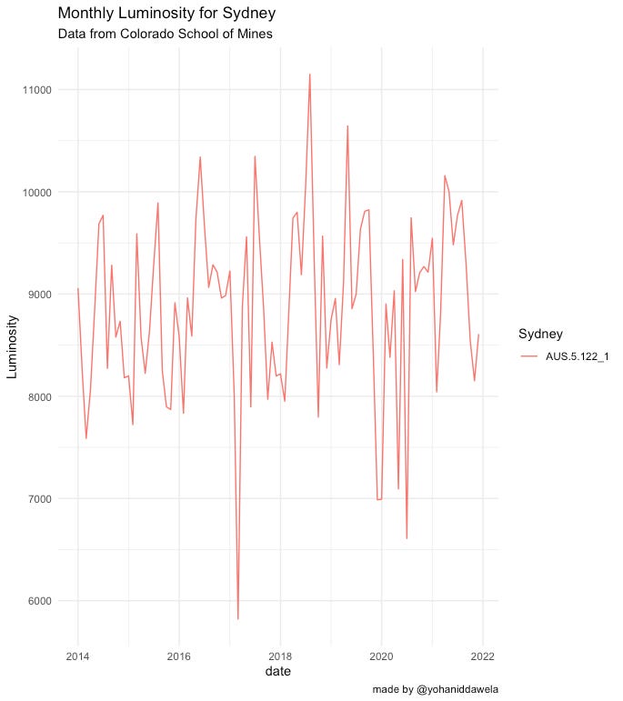
Step 6: Graph the results

We can now create a line graph of monthly luminosity for Sydney using the Colorado School of Mines dataset:

The code to re-produce this graph is as follows:

Step 7: Merging the datasets

Now we simply need to merge the two datasets and re-run the ggplot2 code and we can get something like this, where we can compare the differences between Black Marble and Colorado School of Mines data:

Upon inspecting these two datasets, they seem somewhat consistent with one another.

But if you take the exact same methodology (and codebase), and look at New South Wales, Australia as the region of interest, you’ll see some pretty startling differences (I discuss this in more detail in Part 1).

Conclusion

And there you have it.

A guide to working with Black Marble and Colorado School of Mines nightlights data.

I’ve spent years of my life wrangling these two datasets, so I hope this is a useful shortcut for you all.

And remember, make sure you’re subscribed to get the R scripts delivered to your inbox on 29 December 2023. I’ll only be sending it out once.

UPDATE: As I was putting this guide together, Giacomo Falchetta reached out about his R package blackmaRble, which also helps with querying Black Marble data. You should check it out here: https://github.com/giacfalk/blackmaRble.